Structure of Microscopy Data

Getting familiar with the underlying structure of the package.

In this section, we will dicuss the structure of how spheroid microscopy images can be imported and analysed in SpheroidPy. This functionality is managed in the SpheroidPy.spheroid module. It follows a hierarchical structure, starting from individual (multichannel) images (SpheroidImage), from which multiple timepoints can be combined in a timeseries (SpheroidSeries), from which then in turn multiple replicates can be combined in a collection (SpheroidCollection) for further statistical analysis. Example code accompanying this section is available here.

SpheroidImage  

Individual (multichannel) Microscope Images

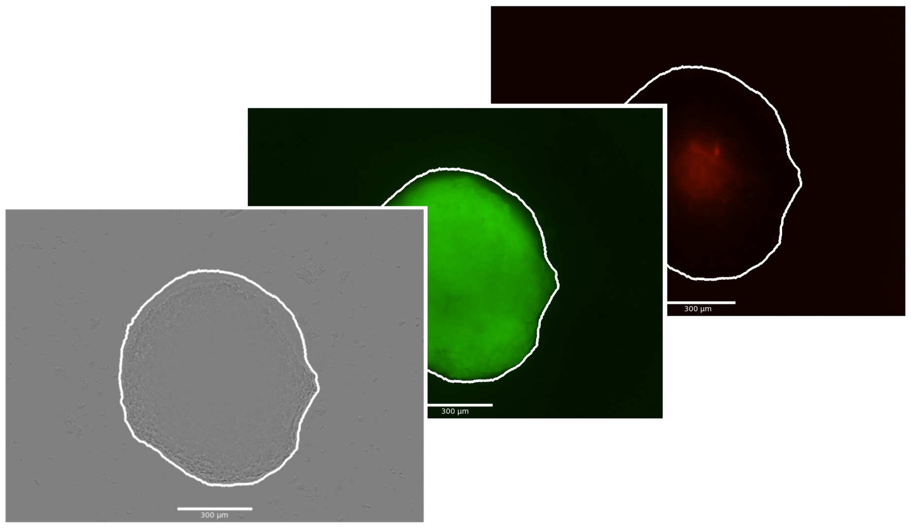
The SpheroidImage class is the most basic building block of SpheroidPy. It manages the microscopy images of different channels for one measurement of a spheroid. After loading the images, they can be segmented using different channels and methods (thresholding or deep learning). In addition, this class implements mathematical methods operating exclusively on the image data, including quantitative analyses based on fluorescence intensities, radial profile computations and biophysical modeling using partial differential equations.

A SpheroidImage can be created by specifying the coresponding image filepaths and the size of the images in both directions.

from SpheroidPy.spheroid import SpheroidImage
my_spheroid = SpheroidImage(brightfield='path/to/brightfield/image', image_size=(x_size,y_size)) # image_size in µm
# additionally also fluorescence channels can be loaded with fluorescence_{color}='path/to/fluorescence/image'

To visualise, whether the creating with the specified images has been successfull, the images can quickly be displayed using the show() method.

my_spheroid.show()  # show all imported images and - if available - the contour

  Note

SpheroidPy supports 4 image channels: a brightfield/phase-contrast and 3 fluorescence (green, red, blue) channels. It supports all common image formats of OpenCV (*.jpeg, *.png, *.tif) and Zeis (*.zvi) and Nikon (*.nd) microscopy formats.

Basic Usage  

Segmentation  

In order to get spatial information from the microscopy images, the contour of the spheroid needs to be determined.

my_spheroid.segmentation(methods=('thresholding','fluorescence_green'), reconstruct_border=True)

# or directly using the respective method:

my_spheroid.segmentation_thresholding(channel='fluorescence_green', thres=1.35) # for thresholding
my_spheroid.segmentation_detectron(channel='brightfield', thres: float = .7) # for AI-based segmentation

  Tip

As it is a frequent problem for live-cell imaging that the spheroids temporarily get out of the field of view (FOV), we have included a method for those incidences. If set true, missing parts of the contour are being reconstructed based on an elliptical shape.

  Important

In order to use the AI-based segmentation pytorch and Detectron2 needs to be installed and the weights have to downloaded to the respective folder. For further information see the installation section.

Metrics  

# based on the contour alone:
my_spheroid.radius, my_spheroid.area
# based on fluorescence channels:
my_spheroid.metric_fluorescence('green')

Advanced Usage  

Methods for the extraction of advanced spatial features resulting from radial inhomogeneities from the spheroid images.

more

Radial Profiles  

Spheroids often develop inhomogeneities represented by radial gradients as the grow, i.e. in cell viability or oxygen/nutrient concentration. Those gradients can often be visualised using fluorescent markers. Accordingly, fluorescence intensity profiles can be extracted as a function of radial distance.

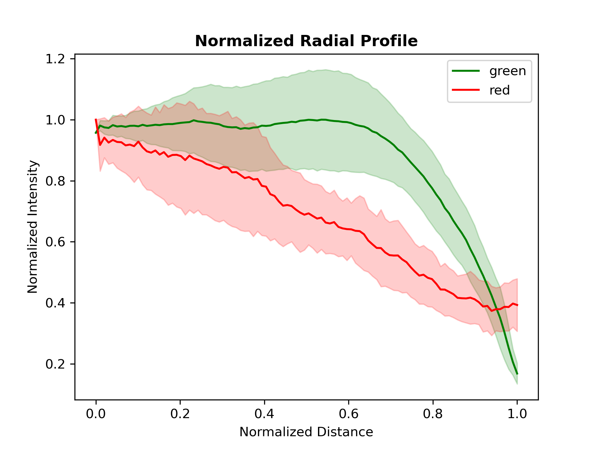
my_spheroid.radial_profile(channels=['green', 'red'], plot=True, angle_step=2)

This method returns a dictionary containing the computed radial intensity profiles for each selected channel, along with the corresponding radial distances.

SpheroidSeries  

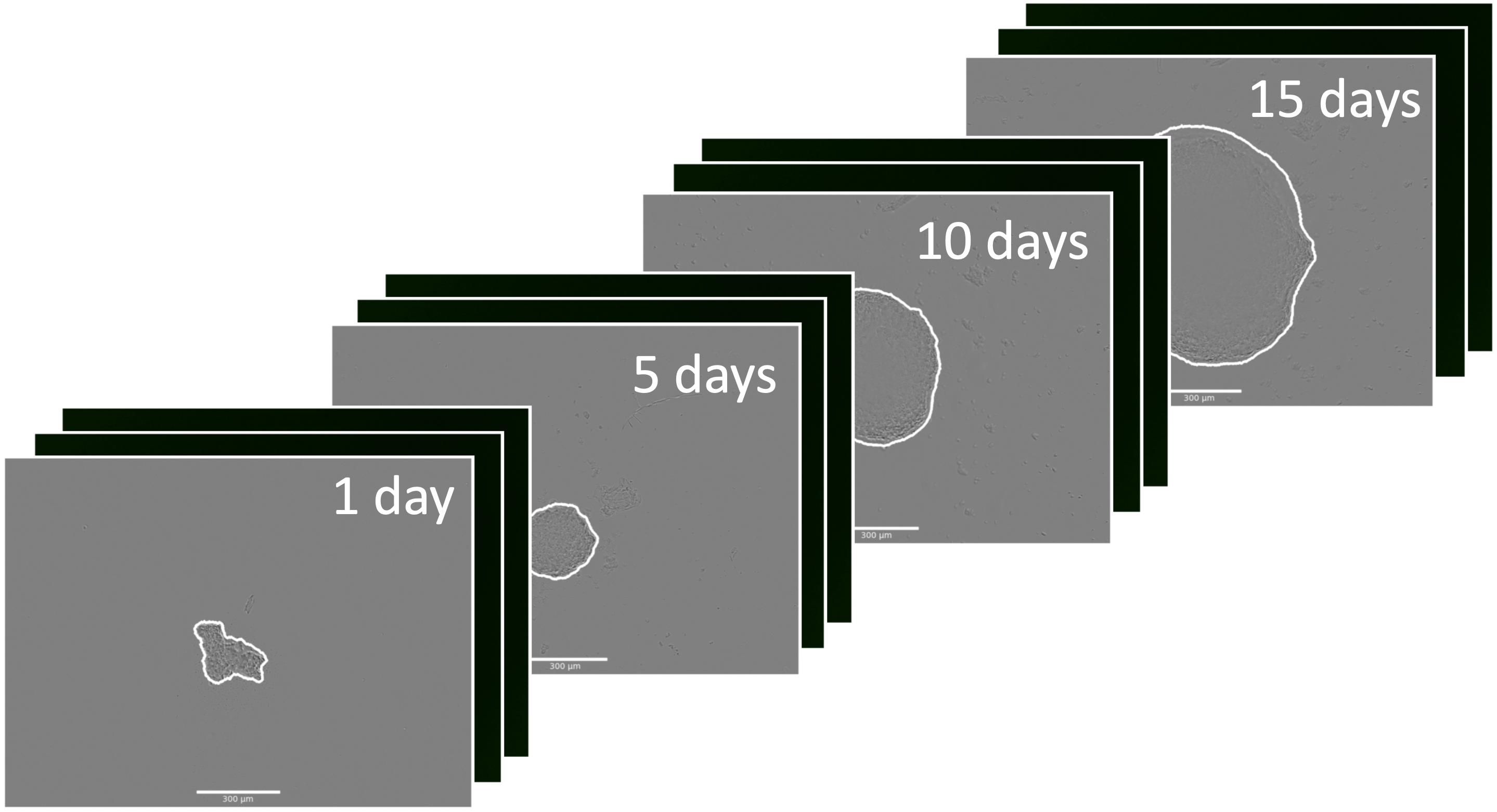
Multiple SpheroidImage instances of the same spheroid at different timepoints can be combined into one SpheroidSeries. This allows for the management of time-lapse microscopy data and investigation of the evolution of the spheroid over time.

from SpheroidPy.spheroid import SpheroidSeries
my_spheroid_series = SpheroidSeries('Name of the Timeseries')

To encount for the timeseries character of the data, the SpheroidSeries has to be associated with multiple SpheroidImages and their respective timepoints. While the SpheroidImages do not contain any time information, this can either be done by iterating over all timepoints and loading the respective files associated with this timepoint.

from datetime import datetime 
# iterate over all timepoints
for day in range(10,25):
    spheroid = SpheroidImage(brightfield = path_bf,
                           fluorescence_green = path_green,
                           fluorescence_red = path_red,
                           image_size = (1700, 1270))
    # specify timepoint
    date_time = datetime.strptime(f'2025y01m{day}d_12h00m','%Yy%mm%dd_%Hh%Mm')
    # add to SpheroidSeries
    my_spheroid_series.add_spheroid_image(spheroid, date_time)

Alternatively, it is also possible to automatically load your data by providing the path to your images as well as filters and automatically let images be assigned to the respective timepoint. While this approach reduces user control over the data loading process it allows for a simpler and more flexible code base. However, it is necessary to keep in mind that this method only works if the nomenclature of the folders or images provides enough information to automatically and correctly detect this information

my_spheroid_series.load_images('path/to/folder', global_filter='Cell_line_A', 
                               brightfield_filter='PhaseContrast', green_filter=['fluo','green'], 
                               red_filter=['fluo','green'], image_size = (1700,1270))

Basic Usage  

Segmentation  

To conveniently perform segmentation of all associated SpheroidImages using the same parameters, a segmentation() method has been implemented in all higher hierarchical classes. This higher-level implementation additionally enables improved performance through multiprocessing capabilities.

my_spheroid_series.segmentation()    # segmentation in all associated SpheroidImages

Visualisation  

All classes provide a built-in show() method that enables convenient and interactive visualization for quality control of image loading and segmentation. Incorrectly segmented spheroids can thus be readily identified, allowing for subsequent re-segmentation with adjusted parameters or alternative methods. As a fallback option, manual segmentation can also be performed.

my_spheroid_series.show()    # opens a widget in jupyter notebook

Basic Metrics  

The temporal evolution of basic quantitative measurements (such as radius, area, or fluorescence intensities) of a SpheroidSeries can be computed using the metric() function.

my_spheroid_series.metric('radius', plot=True) 

This returns the calculated values as a pandas DataFrame for further data analysis in the python ecosystem. If wanted this can also be converted to an Excel file using .to_excel(). If requested also a corresponding plot for visual inspection is provided by the method.

Exporting Videos  

To demonstrate the dynamic of the spheroid growth process, it is possible to export spheroid timeseries as video sequences.

# export video (optional with overlay) as a *.mp4 or *.gif
my_spheroid_series.export_video(
        channel = 'brightfield',
        overlay_channels = ['green', 'red'],
        video_name = 'test.mp4',
        scalebar = True) 

Advanced Usage  

Methods for the extraction of dynamic parameters from the timeseries.

my_spheroid_series.time_period(
    name="treatment_phase",
    start_time="2025-01-16 12:00:00",
    end_time="2025-01-20 12:00:00",
    description="Phase of treatment"
)

SpheroidCollection  

Managing Sets of multiple SpheroidSeries

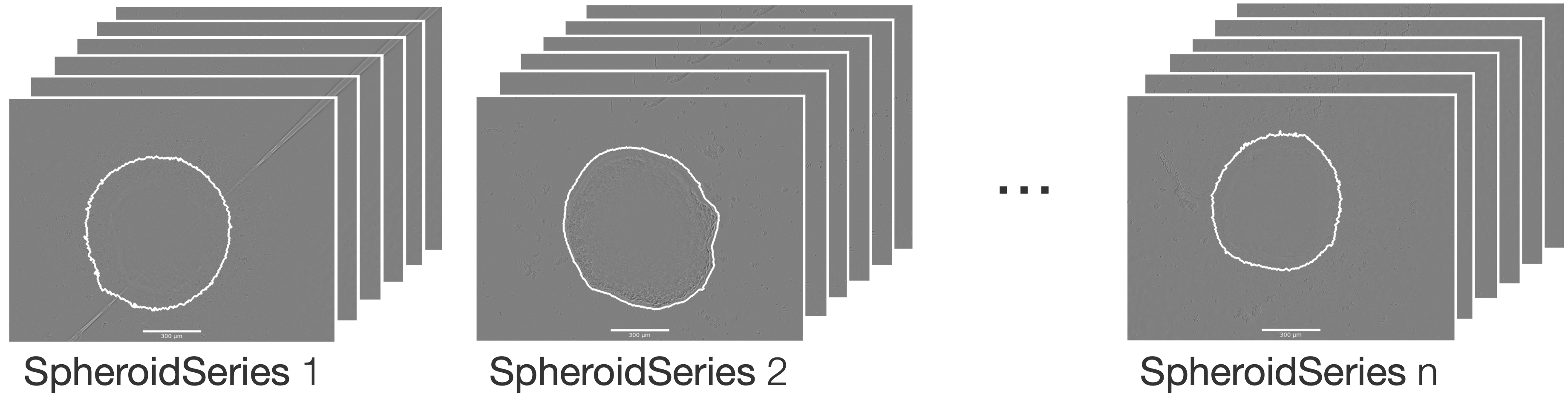
To facilitate the analysis of multiple spheroids, such as technical or biological replicates, several SpheroidSeries can be combined into a single SpheroidCollection. This allows for the calculation of averaged trends, comparison across samples, and simple statistical analyses over the collection.

from SpheroidPy.spheroid import SpheroidCollection
my_spheroid_collection = SpheroidCollection('Name of the collection',
                                            [SpheroidSeries1, SpheroidSeries2, ...])
# or 
my_spheroid_collection = SpheroidCollection('Name of the collection')
my_spheroid_collection.add_series([SpheroidSeries1, SpheroidSeries2, ...])

Basic Usage  

The SpheroidCollection provides the same core methods as the individual series, enabling segmentation, visualisation, and metric extraction with a consistent method interface. This simplifies workflows and supports efficient quality control across multiple SpheroidSeries. The segmentation() and show() methods can be applied to the entire collection.

my_spheroid_collection.segmentation()   # segematation of all associated SpheroidImages
my_spheroid_collection.show()           # display images in an interactive format

In addition to individual calculation, the metric() function also supports statistical evaluation, including calculation of means, standard deviations, and other summary statistics.

my_spheroid_collection.metric('radius', mean=True)

Advanced Usage  

Applying statistical models.